The basic idea of regularisation is to penalise or shrink the large coefficients of a regression model.
This can help with the bias / variance trade-off (shrinking the coefficient estimates can significantly reduce their variance and will improve the prediction error) and can help with model selection by automatically removing irrelevant features (that is, by setting the corresponding coefficient estimates to zero).
Its cons are that this approach may be very demanding computationally.
There are several ways to perform the shrinkage; the regularisations models that we will see are the Ridge regression and the Lasso.
An example: predict credit balanceYou can follow along on the associated notebook.
We will use a small dataset prepared by Stanford’s professors Hastie and Tibshirani.
The Credit data set records Balance (average credit card debt for a number of individuals) as well as several quantitative predictors: age, cards (number of credit cards), education (years of education), income (in thousands of dollars), limit (credit limit), and rating (credit rating).
In addition to these quantitative variables, we also have four qualitative variables: gender, student (student status), status (marital status), and ethnicity (Caucasian, African American or Asian).
The set can be downloaded from the authors’ site or from Kaggle:
import pandas as pd # load up the Credit dataset # data = pd.read_csv("Datasets/credit.csv", index_col=0) data.shape (400, 11) data.columns Index(['Income', 'Limit', 'Rating', 'Cards', 'Age', 'Education', 'Gender', 'Student', 'Married', 'Ethnicity', 'Balance'], dtype='object') Prepare training data: features and targetThe goal is to predict the balance (this is our target variable) based on one or more of the other features.
We start by extracting the target variable:
Suppose that we wish to investigate differences in credit card balance between males and females, ignoring the other variables for the moment.
If a qualitative predictor has only two levels then we can simply create an indicator or dummy variable that takes on two possible numerical values.
We can use the Python map() primitive to map Female to 1 and Male to 0.
Be careful that the labels need to be mapped correctly, eventual spaces included.
The decision to use 0 or 1 is arbitrary and has no effect on the regression fit but different values could result in different coefficients.
We now use the new dummy variable as a predictor in a regression model.
from sklearn import linear_model # # Create the linear regression model # model = linear_model.LinearRegression() model.fit(X[['Gender']], y) model.intercept_ 509.80310880829012 model.coef_ array([ 19.73312308])This results in the model:
Balance = $509.7 if male
Balance = $509.7 + $19.7 if female
And 19.7 can be interpreted as the average difference in credit card balance between females and males (females are estimated to carry $19.7 in additional debt for a total of 509.7+19.7 = $529.4).
However without checking its p-value or confidence intervals (outside the scope of this) we cannot say anything about the statistical evidence of this difference.
When a qualitative predictor has more than two levels, a single dummy variable cannot represent all possible values. In this situation, we can split a categorical variable into additional different binary variables, one for each level.
For example, for the ethnicity variable we create three dummy variables, using the pandas function get_dummies().
Since the dummies variable are additional – not new values mapped to the existing variable like for the gender – we can now drop the Ethnicity variable:
X.drop(['Ethnicity'], axis=1, inplace=True) features = X[['Asian', 'Caucasian', 'African American']] model.fit(features, y) model.intercept_ 520.60373764246071 model.coef_ array([ -8.29001215, -2.10625021, 10.39626236])We see that the estimated balance for the African American is $531.00 = 520.60 + 10.40; it is estimated that the Asian category will have 18.7 dollars less debt than the African American category, and that the Caucasian category will have $12.50 less debt than the African American category.
Again, no statistical evidence.
Predict from all variablesFirst we convert the other two categorical variables:
X.Student = X.Student.map({'Yes':1, 'No':0}) X.Married = X.Married.map({'Yes':1, 'No':0})Now we implement a naive version of the Forward Stepwise Selection:
start from a null model and add the next feature with the best score (in terms of square error).
The first features are Rating, Limit, Income and Student.
Just with these 4 features, the R2 score is already at 0.95
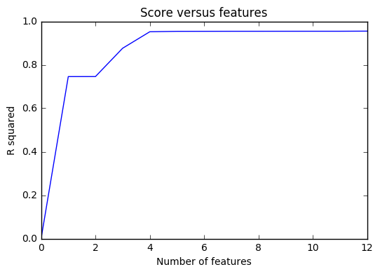
The first four features are the best predictors, the others do not add too much value.
As we add more and more parameters to our model its complexity increases, which results in increasing variance and decreasing bias, i.e. overfitting.
Basically there are two methods to overcome overfitting,
- Reduce the model complexity (less features! Use a selection algorithm as the one above and extract a subset of features).
- Regularisation (what we are going to see now)
The subset selection methods use least squares to fit a linear model that contains a subset of the predictors.
As an alternative, we can fit a model containing all p predictors using a technique that constrains or regularises the coefficient estimates.
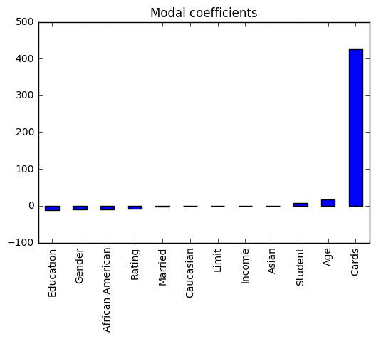
We can see that the coefficient of Card is much higher as compared to rest of the coefficients. Therefore the credit balance of a person would be more driven by this feature.
Ridge regressionRecall that the least squares fitting procedure estimates the beta coefficients using the values that minimise

Ridge regression is very similar except that the beta coefficients are estimated by minimising

As with least squares, ridge regression seeks coefficient estimates that fit the data well, by making the RSS small. However it adds a second term, called a shrinkage penalty, where lambda is a tuning parameter, to be determined separately.
If lambda = 0 then the formula is like least squares but as lambda grows the impact of the shrinkage penalty grows and the beta coefficients will approach zero (shrinking).
SKlearn has a module Ridge to apply a ridge regression model.
Let’s see an example using lambda = 0.05 (called alpha in SciKitLearn)
As you can see, the coefficients have been shrunk, and Cards is not sticking out anymore.
StandardiseThe least squares coefficient estimates are scale equivariant: multiplying X by a constant c simply leads to a scaling of the least squares coefficient estimates by a factor of 1/c.
In contrast, the ridge regression coefficient estimates can change substantially when multiplying a given predictor by a constant, due to the sum of squared coefficients term in the penalty part of the ridge regression objective function.
Therefore, it is best to apply ridge regression after standardising the predictors.
Let’s plot the coefficients values based on the lambda parameter λ.
import numpy as np lambdas = [0.01, 1, 100, 10000] coefficients = np.zeros(shape=(12, len(lambdas))) i=0 for l in lambdas: ridgeReg = Ridge(alpha=l) ridgeReg.fit(X, y) coefficients[:,i] = ridgeReg.coef_ i += 1 fig, ax = plt.subplots() plt.title("Ridge regularisation") plt.xlabel("lambda") plt.ylabel("standardised coefficients") styles=['-','--','-.',':'] labels = ['0.01','','1','', '100','', '1e4',''] ax.set_xticklabels(labels) # custom x labels for i in range(0,12): s = styles[i % len(styles)] if i<3 or i==7: plt.plot(coefficients[i], label=predictors[i], linestyle=s) else: plt.plot(coefficients[i]) plt.legend(loc='best')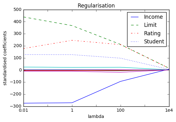
Each curve corresponds to the ridge regression coefficient estimate for one of the variables, plotted as a function of λ.
At the left side of the plot, λ is essentially zero, and so the corresponding ridge coefficient estimates are the same as the usual least squares estimates. But as λ increases, the ridge coefficient estimates shrink towards zero. When λ is extremely large, then all of the ridge coefficient estimates are basically zero; this corresponds to the null model that contains no predictors.
In this plot, the income, limit, rating, and student variables are displayed in distinct colours, since these variables are the ones to have the largest coefficient estimates.
Why Does Ridge Regression Improve Over Least Squares?
Ridge regression’s advantage over least squares is rooted in the bias-variance trade-off.
As λ increases, the shrinkage of the ridge coefficient estimates leads to a substantial reduction in the variance of the predictions, at the expense of a slight increase in bias.
Therefore ridge regression works best in situations where the least squares estimates have high variance.
Ridge regression also has substantial computational advantages over best subset selection, which requires searching through 2p models.
Ridge regression does have one obvious disadvantage.
Unlike best subset, forward stepwise, and backward stepwise selection, which will generally select models that involve just a subset of the variables, ridge regression will include all p predictors in the final model.
The penalty λ will shrink all of the coefficients towards zero, but it will not set any of them exactly to zero.
This may not be a problem for prediction accuracy, but it can create a challenge in model interpretation in settings in which the number of variables p is quite large.
For example, in the Credit data set, it appears that the most important variables are income, limit, rating, and student. So we might wish to build a model including just these predictors. However, ridge regression will always generate a model involving all ten predictors.
Increasing the value of λ will tend to reduce the magnitudes of the coefficients, but will not result in exclusion of any of the variables. The lasso is a relatively recent alternative to ridge regression that over-comes this disadvantage.
The lasso coefficients minimise the quantity
$latex RSS + \lambda \sum_{j=1}^{p}\left | \beta _{j} \right | &s=3$
from sklearn.linear_model import Lasso lassoReg = Lasso(alpha=0.3) lassoReg.fit(X, y) Lasso(alpha=0.3, copy_X=True, fit_intercept=True, max_iter=1000, normalize=False, positive=False, precompute=False, random_state=None, selection='cyclic', tol=0.0001, warm_start=False) lassoReg.score(X, y) 0.95509337268728689In statistical parlance, the lasso uses an L1 penalty instead of an L2 penalty.
The L1 penalty has the effect of forcing some of the coefficient estimates to be exactly equal to zero when the tuning parameter λ is sufficiently large. Hence, much like best subset selection, the lasso performs variable selection.
As a result, models generated from the lasso are generally much easier to interpret than those produced by ridge regression.
The lasso yields sparse models — that is, models that involve only a subset of the variables.
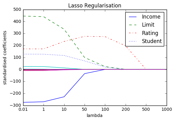
When λ = 0, the lasso simply gives the least squares fit and when λ becomes sufficiently large, the lasso gives the null model in which all coefficient estimates equal zero.
However, in between these two extremes, the ridge regression and lasso models are quite different from each other, as you can see from the two plots.
Both in ridge regression and lasso, the tuning parameter serves to control the relative impact of the shrinking terms on the regression coeffcient estimates.
Selecting a good value for λ is critical; cross-validation is used for this.
Cross-validation provides a simple way to tackle this problem. We choose a grid of λ values, and compute the cross-validation error for each value of λ
We then select the tuning parameter value for which the cross-validation error is smallest.
Finally, the model is re-fit using all of the available observations and the selected value of the tuning parameter.
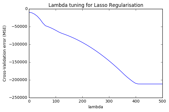
The plot displays how the cross-validation error changes with different values of lambda. The point at which the cross-validation error is smallest is for very small values of lambda, close to zero.
Thanks to the sklearn function LassoCV, that applies cross-validation to the Lasso, we can calculate the exact value of lambda that minimise the error:
This post is part of a series about Machine Learning with Python.
Advertisements Share this:- More


