As a side activity, I do some sports betting. After 2.5 years of using the so-called draw strategy in football bettings, I now decided to evaluate my betting performance using R. In order to show also the technical details to the analysis, I'll incude my code as usual in this blog. But for privacy reasons, I will not publish the data behind the analysis. Thus, you cannot run the analysis on my data, but I hope you will be able to follow the way I worked anyway.
The strategyI found the betting strategy here and decided to give it a try. I slightly adapted the strategy and do the following:
I choose teams (mostly with a balanced goal difference) and bet on draws in each round. If a game has a winner, I bet on draw for the same team in the next game and increase the wager with factor 1.5. This is repeated until the team plays draw, which ensures that I have a profit after each successful bet. After a draw, I start again with my initial wager. This progressive betting system is extremely risky, since the wager can get extremely high after several unsuccessful rounds. Thus, I remind myself to stick to some vital rules (see below under Conclusions) in order not to go bankrupt.
My betting performanceI have played about 1,000 bets at this point, which enables me to get some interesting insights through data analysis. First, I'll do the analytical part and look for profits, success rates and rates of return:
total_bets <- read.csv('D:/Daniel/Blog/Daten/evaluation_betting_on_draws.csv', header = TRUE, sep = ";", dec = ",") total_profit <- sum(total_bets$Profit) total_wager <- sum(total_bets$Wager) total_games <- as.data.frame(count(total_bets, "Result")) profit_per_game <- total_profit / total_games$n total_rate_of_return <- (total_profit / total_wager) * 100 profit_season <- total_bets %>% group_by(Season) %>% summarise(sum(Profit)) wager_season <- total_bets %>% group_by(Season) %>% summarise(sum(Wager)) games_per_season <- total_bets %>% count(Season) %>% group_by(Season) profit_League <- total_bets %>% group_by(League) %>% summarise(sum(Profit)) wager_League <- total_bets %>% group_by(League) %>% summarise(sum(Wager)) games_per_League <- total_bets %>% count(League) %>% group_by(League) profit_season <- as.data.frame(profit_season) wager_season <- as.data.frame(wager_season) games_per_season <- as.data.frame(games_per_season) table_season <- merge(profit_season, games_per_season, by = "Season") table_season <- merge(table_season, wager_season, by = "Season") profit_League <- as.data.frame(profit_League) wager_League <- as.data.frame(wager_League) games_per_League <- as.data.frame((games_per_League)) table_League <- merge(profit_League, games_per_League, by = "League") table_League <- merge(table_League, wager_League, by = "League") table_season$profit_per_game <- table_season$"sum(Profit)" / table_season$n ### success rates total_success_rate <- total_bets %>% count(Result) %>% mutate(freq = n / sum(n)) success_rate_season <- total_bets %>% count(Result, Season) %>% group_by(Season) %>% mutate(freq = n / sum(n)) success_rate_league <- total_bets %>% count(Result, League) %>% group_by(League) %>% mutate(freq = n / sum(n)) ### rate of return table_season$rate_of_return <- (table_season$"sum(Profit)" / table_season$"sum(Wager)") table_League$rate_of_return <- (table_League$"sum(Profit)" / table_League$"sum(Wager)") ### merge success rates and rate of return by season success_rate_season1 <- as.data.frame(success_rate_season) table_merge_season <- subset(table_season[, c(1, 6)]) table_merge_season$success_rate <- subset(success_rate_season1[, c(4)], success_rate_season1$Result == 1) table_merge_season$var1 <- c("Rate of return") table_merge_season$var2 <- c("Success rate") table_merge_ror <- subset(table_merge_season[, c(1, 2, 4)]) table_merge_succrate <- subset(table_merge_season[, c(1, 3, 5)]) table_merge_season <- rbindlist(list(table_merge_succrate, table_merge_ror)) table_merge_season$var2 <- factor(table_merge_season$var2, levels = c("Success rate", "Rate of return")) # change sequence of Succress rate and rate of return for plot ### merge success rates and rate of return by league success_rate_league1 <- as.data.frame(success_rate_league) table_merge_league <- subset(table_League[, c(1, 5)]) table_merge_league$success_rate <- subset(success_rate_league1[, c(4)], success_rate_league1$Result == 1) table_merge_league$var1 <- c("Rate of return") table_merge_league$var2 <- c("Success rate") table_merge_league_ror <- subset(table_merge_league[, c(1, 2, 4)]) table_merge_league_succrate <- subset(table_merge_league[, c(1, 3, 5)]) table_merge_league <- rbindlist(list(table_merge_league_succrate, table_merge_league_ror)) table_merge_league$var <- factor(table_merge_league$var, levels = c("Success rate", "Rate of return")) # change sequence of Succress rate and rate of return for plotOverall, I bet on exactly 1,013 games and had a success rate of 35.8%. Using my betting strategy explained above, this led to an overall rate of return (or return of investment) of 20.2%. As you can see in the plot below, there are quite large differences by seasons. The current season 2017/18 is by far the most successful until now when looking at the share of games I bet on and which actually ended draw (success rate of 38.8%). This is also the first season I decided only to bet on the Italian Serie B after splitting my bets in different leagues in the first two years. It turned out that teams in this league have a higher probability of playing draw than teams in other leagues (39% of all games I bet on in the Italian Serie B ended draw).
I won 35.1% of my games in season 2016/17 and 32.5% in the season 2015/16. It is nice to see that there is an obvious learning curve. Looking at the rate of return, I had a really weak season 2016/17 (14.5%) compared to 2015/16 (27.5%) and 2017/18 (24%). This finding is interesting, since a higher success rate is apparently not automatically leading to a higher rate of return. The reason for this is that high losses in losing teams (in my case the French Ligue 2) have to be compensated by winning teams before having profits. This result shows that a high success rate is not automatically efficient when running a progressive betting system.
ggplot(table_merge_season) + geom_bar(aes(x = Season, y = success_rate, fill = var2), position = 'dodge', stat = 'identity', width = 0.4, color = 'cyan') + labs(x = 'Season', y = 'Share of games won / Rate of return', title = "Success rate of bets on draws by season") + scale_y_continuous(labels = scales::percent) + scale_fill_manual("", values = c("Rate of return" = "steelblue", "Success rate" = "steelblue4")) + theme(text = element_text(family = 'Gill Sans', color = "#444444"), panel.background = element_rect(fill = '#444B5A'), panel.grid.minor = element_line(color = '#4d5566'), panel.grid.major = element_line(color = '#586174'), plot.title = element_text(size = 18, hjust=0.5), axis.title = element_text(size = 16, color = '#555555'), axis.title.y = element_text(vjust = 3), axis.title.x = element_text(hjust = 0.5), axis.text.x = element_text(size = 12), axis.text.y = element_text(size = 12), legend.text = element_text(size = 12) )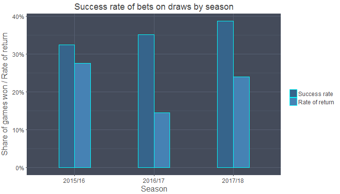
The data analysed by league show some suprising results, although they are skewed by the fact that some leagues have only few observations compared to others. E.g., I bet on 630 games in the Italien Serie B and only a few in the German 1. Bundesliga (38) or the English Premiere League (40) and Championship (29). It seems that I was extremely lucky with my choices in the leagues with few observations, since I had very high rates of return in the Premiere League (42.7%), the 1. Bundesliga (40.9%) and the Championship (39.3%). Regarding the large number of games played, I was also quite successful in the Italian Serie B, where I was able to achieve a rate of return of 27.1%. I performed really bad in my short betting history on teams of the French Ligue 2 (-15.3%), while the rate of return of 14.8% for the 2. Bundesliga was more or less ok. My success rate on teams of the Serie B is extremely high with 39.7%, but some bad performing teams lower my rate of return here. The following plot summarizes the results by league:
ggplot(table_merge_league) + geom_bar(aes(x = League, y = success_rate, fill = var), position = 'dodge', stat = 'identity', width = 0.4, color = 'cyan') + labs(x = 'League', y = 'Share of games won / Rate of return', title = "Success rate of bets on draws by league") + scale_y_continuous(labels = scales::percent) + scale_fill_manual("", values = c("Rate of return" = "steelblue", "Success rate" = "steelblue4")) + theme(text = element_text(family = 'Gill Sans', color = "#444444"), panel.background = element_rect(fill = '#444B5A'), panel.grid.minor = element_line(color = '#4d5566'), panel.grid.major = element_line(color = '#586174'), plot.title = element_text(size = 18, hjust=0.5), axis.title = element_text(size = 16, color = '#555555'), axis.title.y = element_text(vjust = 3), axis.title.x = element_text(hjust = 0.5), axis.text.x = element_text(size = 12), axis.text.y = element_text(size = 12), legend.text = element_text(size = 12) )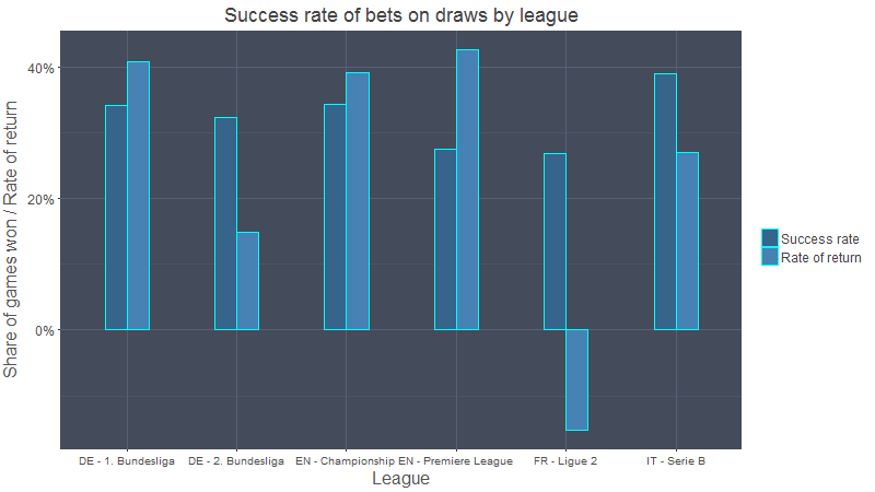
The results show me that it would be better to have a good mix of teams in different leagues, as I had in season 2015/16 instead of betting a whole league as I do now. But the season 2016/17 showed me that the team selection is tricky and can be a complete flop. Thus, I stick with my current selection, having a rate of return of 24% (which I think is pretty good) and add some additional teams with high shares of games played draws. In midseason, the values should be reliable overall. E.g. I'll include my Premiere League strategy I had last season, where I bet on each game between the big six teams (Manchester United, Manchester City, Arsenal London, Chelsea London, Liverpool FC and Tottenham Hotspurs). I had a success rate of 35.3% in these games (average odds: 3.44, which suggests that less than 30% of the games end draw) and a rate of return of 45.6%(!).
Some deeper analysisAfter this analysis, I decided to make an evaluation of historical football results in the Serie B in Italy. My hope was to find some interesting patterns, which help me to improve my betting performance. I found the historical data on this portal and downloaded them.
files <- list.files('D:/Daniel/Serie_B', pattern='*.csv') SerieB <- files %>% map_df(~ read.csv(file.path('D:/Daniel/Serie_B', .))) SerieB <- subset(SerieB, SerieB$Date != "") colnames(SerieB) SerieB <- select(SerieB, c(1:19, 23:25, 46:48)) colnames(SerieB) SerieB$month <- substr(SerieB$Date, start=4, stop=5) names(SerieB) <- c('Division', 'Date', 'HomeTeam', 'AwayTeam', 'HomeTeamGoals', 'AwayTeamGoals', 'Result', 'HT_HomeTeamGoals', 'HT_AwayTeamGoals', 'HT_Result', 'GB_HomeWinOdds', 'GB_DrawOdds', 'GB_AwayWinOdds', 'Interwetten_HomeWinOdds', 'Interwetten_DrawOdds','Interwetten_AwayWinOdds', 'WilliamHill_HomeWinOdds', 'WilliamHill_DrawOdds','WilliamHill_AwayWinOdds', 'Bet365_HomeWinOdds','Bet365_DrawOdds','Bet365_AwayWinOdds','BWin_HomeWinOdds', 'BWin_DrawOdds','BWin_AwayWinOdds') SerieB$Season <- c('Season1997/98') SerieB$Season[8124:8503] <- c('Season1998/99') SerieB$Season[8504:8883] <- c('Season1999/00') SerieB$Season[1:380] <- c('Season2000/01') SerieB$Season[381:751] <- c('Season2001/02') SerieB$Season[752:1140] <- c('Season2002/03') SerieB$Season[1141:1692] <- c('Season2003/04') SerieB$Season[1693:2154] <- c('Season2004/05') SerieB$Season[2155:2616] <- c('Season2005/06') SerieB$Season[2617:3078] <- c('Season2006/07') SerieB$Season[3079:3540] <- c('Season2007/08') SerieB$Season[3541:4002] <- c('Season2008/09') SerieB$Season[4003:4464] <- c('Season2009/10') SerieB$Season[4465:4926] <- c('Season2010/11') SerieB$Season[4927:5388] <- c('Season2011/12') SerieB$Season[5389:5850] <- c('Season2012/13') SerieB$Season[5851:6312] <- c('Season2013/14') SerieB$Season[6313:6774] <- c('Season2014/15') SerieB$Season[6775:7236] <- c('Season2015/16') SerieB$Season[7237:7698] <- c('Season2016/17') SerieB$Season[7699:7743] <- c('Season2017/18')As can be seen in the plot below, more than 30% of all games played in the league ended in a draw in most seasons (I included data from 1997/98 until the running season 2017/18).
ggplot(table_results_season, aes(x=Season, y=freq, linetype=Result, group=Result)) + geom_line(color = 'cyan', size=1) + labs(x = 'Season' , y = 'Percentage', title = "Shares of each result in Italian SerieB by season") + theme(text = element_text(family = 'Gill Sans', color = "#444444"), panel.background = element_rect(fill = '#444B5A'), panel.grid.minor = element_line(color = '#4d5566'), panel.grid.major = element_line(color = '#586174'), plot.title = element_text(size = 20, hjust=0.5), axis.title = element_text(size = 16, color = '#555555'), axis.title.y = element_text(vjust = 0.5), axis.title.x = element_text(hjust = 0.5), axis.text.x = element_text(size = 12), axis.text.y = element_text(size = 12), legend.text = element_text(size = 12) )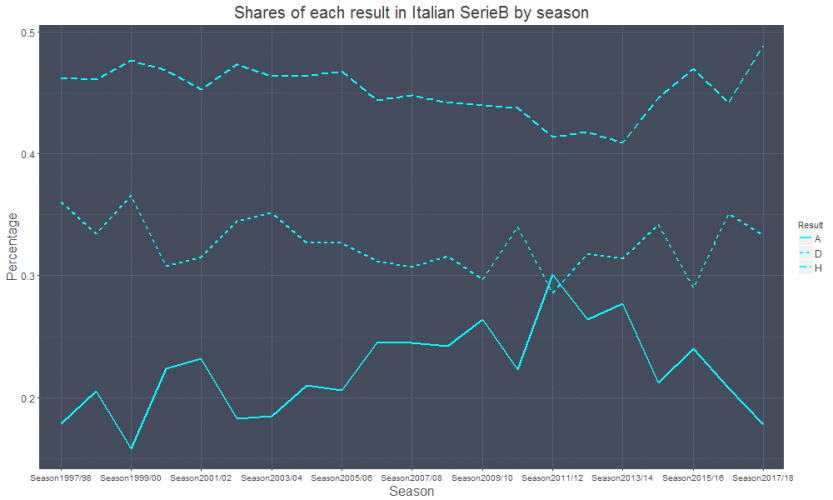
Interestingly, there is a clear difference in the shares of results with respect to the playing period. Draws are especially probable at the start of the season in August, in December (christmas peace?) and at the end of the season, when many clubs already consolidated their position in the league. This is also the period, when (in relative terms) most away wins happen. Especiall May seems to be a bad month for betting on draws, which is shown in the following figure.
ggplot(table_results_month, aes(x=month, y=freq, linetype=Result, group=Result)) + geom_line(color = 'cyan', size=1) + labs(x = 'Month' , y = 'Percentage', title = "Shares of each result in Italian SerieB per Month") + theme(text = element_text(family = 'Gill Sans', color = "#444444"), panel.background = element_rect(fill = '#444B5A'), panel.grid.minor = element_line(color = '#4d5566'), panel.grid.major = element_line(color = '#586174'), plot.title = element_text(size = 20, hjust=0.5), axis.title = element_text(size = 16, color = '#555555'), axis.title.y = element_text(vjust = 0.5), axis.title.x = element_text(hjust = 0.5), axis.text.x = element_text(size = 12), axis.text.y = element_text(size = 12), legend.text = element_text(size = 12) )
This naturally also affects betting odds, which are slightly higher in May and lower in June.
ggplot(SerieB[SerieB$Result=='D',], aes(y=Interwetten_DrawOdds,x=month))+ geom_boxplot(color = 'cyan') + ylim(0,6) + labs(x = '' , y = 'Draw Odds', title = "Draw Odds vs. Results per Month") + theme(text = element_text(family = 'Gill Sans', color = "#444444"), panel.background = element_rect(fill = '#444B5A'), panel.grid.minor = element_line(color = '#4d5566'), panel.grid.major = element_line(color = '#586174'), plot.title = element_text(size = 20, hjust=0.5), axis.title = element_text(size = 16, color = '#555555'), axis.title.y = element_text(vjust = 0.5), axis.title.x = element_text(hjust = 0.5), axis.text.x = element_text(size = 12), axis.text.y = element_text(size = 12), legend.text = element_text(size = 12) )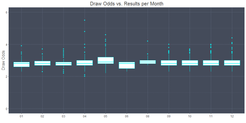
In order to improve my betting system, I wanted to know which odds appeared most often when a certain result happened. Thus, I used boxplots and their characteristics to analyze this. First, I summarized the home win odds from all games in the dataset and calculated the minimum, lower quartile, median, upper quartile and maximum for each result.
result_boxplot_homewin ## A D H ## min 1.3 1.05 1.03 ## lower quartile 2.0 1.85 1.70 ## median 2.2 2.10 2.00 ## upper quartile 2.6 2.40 2.30 ## max 3.5 3.20 3.10I did the same for the away win odds:
result_boxplot_awaywin ## A D H ## min 1.25 1.25 1.4 ## lower quartile 2.70 2.90 3.0 ## median 3.10 3.30 3.7 ## upper quartile 3.70 4.20 4.6 ## max 5.20 6.00 6.8And also the draw odds:
result_boxplot ## A D H ## min 2.50 2.3 2.3 ## lower quartile 2.70 2.7 2.7 ## median 2.80 2.8 2.8 ## upper quartile 2.90 3.0 3.0 ## max 3.15 3.4 3.4According to this, I set the following thresholds for my bets:
- Odds of home team larger than 1,8 and smaller than 2,45
- Odds of away team larger than 2,8 and smaller than 4,25
- Odds for a draw larger than 2,7 and smaller than 3,25
It turned out that in the first 20 rounds of the season 2017/2018, betting using the thresholds above would not have improved my betting performance. My success rate was higher by about 15% when simply betting games, which had draw odds lower than 3.4 (as stated above, my success rate for the first half of season 2017/2018 in the Italien Serie B is 38.8%).
ConclusionThe rate of return for this betting strategy shows me that it is highly profitable. Nonetheless, I'm fully aware that this progressive betting strategy is highly risky and that one team not playing draw a long time can cost me all the money I invested in this system. I was able to make some nice profit over the years following some clear rules:
-
Start with an amount of risk capital which you can afford to lose and do not re-buy. The amount of money must be chosen carefully and it should not affect your life if it is lost. From my experience, your starting capital should be about a hundred times the amount of the inital wager of the first bet (assuming you bet on about 20 teams). I also had situations where I had to spend more money than I had on my betting account. In these cases, I held firm to my strategy and bet on the same games I would have done with more money. But in order to do this, I splitted the remaining money and simply bet less than it should have been. Fortunatly, this strategy was successful and I was able to get out of the hole and increase my account again. Be aware that this is a process which takes time.
-
Realize your profits. If you're winning – in my experience, I start to win in November after some holes in the first two months – collect your gains until your starting capital threshold. This ensures that you do not lose all your profits if you have a bad period. If you lose all your money at some point in a season, don't rebuy and feed the bookies! Instead, be happy with the money you already got out.
-
Do not bet every game. As stated in the strategy I followed (see link here), it can be useful to take into account home and away games and other influence factors.
-
Stop betting on one team, when a certain threshold of wager is reached. Increasing the wager with factor 1.5 every time a team is not playing draw can lead to huge amounts of money. Even if you lose with one of your teams, it may be more profitable to stop betting on this team and focusing on the profitable ones. The decision on when to stop betting on a team is tough, since the next game can be the one with a draw and make your profits jump. Be aware that it also can cost you all your profits from other teams if you don't stop betting on the bad teams.