In our previous post, we understood in detail about Linear Regression where we predict a continuous variable as a linear function of input variables. But in case of the binomial variable, we follow another approach called Logistic regression where we predict the probability of the output variable as a logistic function of the input variable. Logistic regression is majorly used for classification problem and we can also understand it from the neural network perspective. In this post, I will explain how logistic regression can be used as a building block for the neural network.
The first step in this procedure is to understand Logistic regression.
Unlike Linear Regression, Logistic Regression forms a model which gives the predicted probability of target variable as a function of input variable X. So, if we consider if X as an input vector then we would want to predict whether particular observation belongs to either class “0” or class “1” (in case of binary classification).
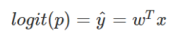
We know that linear regression can be expressed by below equation:
yᶺ = wT .x
But apparently, this equation does not work well in case of binary classification because we want yᶺ to be the chance that y =1 or 0. If we use linear regression for classification problem our linear regression model will not perform well because of many reasons.
First, linear regression model which is used to predict the continuous variable assumes the target variable to be normally distributed. However, in case of classification problem where the target variable is 0 and 1 this assumption is clearly violated. Secondly, in classification problem where we are predicting the probability of target variable, linear regression will give us values which are above 1 and below 0. Also, the predictions made using linear regression can be highly inaccurate. This is when sigmoid function comes into the picture. The sigmoid function helps in bringing non-linearity in the model. As we are predicting the probability of class 0 and 1 we would not want it to be less than 0 and more than 1. Sigmoid function helps in bounding the probability between 0 and 1. Also, since the derivative of a sigmoid function is easy to calculate we can further use that in the neural network.
In Logistic regression, the logistic function can be given as –
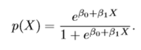
Here, P(X) is nothing but the probability of y =1 given the input vector X.
This can be further expressed as –

Here, the first term in above equation is termed as odds and it can take any value between 0 to ∞. So, to bound its value between 0 and 1, we take log on both the sides of above equation.
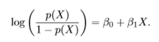
The left-hand side of above equation is called as log-odds or logit and the right-hand side of the equation is now similar to our linear regression. Thus, although non-linear in x, log odds of logistic is linear in X.
As we can see the logit function act as a link between logistic regression and linear regression and hence it is also called as a link function.
Our next step would be to calculate weights w which I will explain after we derive sigmoid function. Once the weights are estimated we take the inverse of logit function to find the probability p.

Adding 1 on both sides of above equation
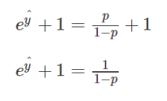
This can also be written as-
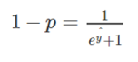
Subtracting 1 from both sides of equation-

Multiplying both sides by -1
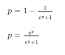
Dividing both numerator and denominator by eyᶺ
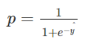
The above equation represents a sigmoid function which is used in logistic regression and it is denoted by σ.
Hence the final logistic regression equation will look like this
yᶺ = σ (wT.x + b)
for simplicity let us denote wT.x + b = z
yᶺ = σ (z)
σ (z) = 1/1+ e-z
If the value of z is very large positive number then
σ (z) = 1/1+0
= 1
And if the value of z is very large negative number then
σ (z) = 1/1+ (big number)
and σ (z) will approximate to 0
So, we can see that the value is bound between 0 and 1.
Now to train our model we need to define the cost function for our logistic regression problem.
Before looking at cost function let us see the loss function of logistic regression.
The loss function is nothing but the error function which will tell us how good our output variable y^ is when the true label is y.
We generally use squared error method to find the loss function but in logistic regression, this method does not work well for gradient descent. Hence, we will define different loss function which plays a similar role like a squared error (for linear regression) and will give us optimization curve which will be convex in shape.
So, the loss function for logistic regression is given as-
L(y^,y) = -(y log y^ + (1-y) log(1- y^))
Here we want our loss function to be minimum just like the squared error function in Linear regression.
The key point here is Loss function is given for single training example. When we calculate the error for entire training set it is given my Cost function.
So, the cost function which is applied to entire training set is given as-
J (w, b) = 1/m * sum(L(y^,y) ( for all the observation in training dataset.)
J (w, b) = -1/m * sum ( y(i).log(y^(i)) + (1- y(i)).log(1- y^(i)))
So, our aim is to find the parameter w and b that minimizes the overall cost function of the model
From here we can implement logistic regression in the form of single neural network (NN). We will see how we can use gradient descent to find w for our dataset which is called back propagation in this case. The intuition behind gradient descent is explained in one of our previous post which can be found here.
We will understand this with the help of computation graph.
In this graph, we follow a forward path propagation where we find the output of neural network and this will be followed by backward propagation where we find the gradient.
Let us assume that we only have two input variables(x1,x2) in our training dataset. Therefore, to find the output we will have to introduce weights of these variables and b, which have to be found using gradient descent. This can be better explained by computational graph given below-
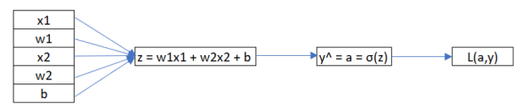
Forward Propagation:
Step 1: Multiply the weights and input variable for a given training set and add bias to the equation. The final equation will be denoted by z.
z = w1x1 + w2x2 + b
Step 2: Multiply z with the activation function. We are using sigmoid function denoted by σ as the activation function. However, there are different activation functions we can use for the same purpose. The gradient and the value of weights will change with respect to the activation function. This multiplication will yield the predicted value of y, denoted by a.
y^ = a = σ(z)
Step 3: The final step is to calculate the error function which is nothing but our loss function, denoted by L. This function will denote the error between our predicted value and the actual value which is our final output of the neural network.
L(a ,y) = -(y log a + (1-y) log(1- a))
Backward propagation:
In backward propagation, we find the gradient or derivative of the loss function (L(a, y)) with respect to the weights. Since we are interested in finding gradient here we will follow backward propagation.
Here, z represents the linear regression equation which when multiplied with the sigmoid function (activation function) will yield the predicted value of y, denoted by a. (Note: The proof of derivatives used in following steps will be given at the end of this article)
Step 1: Compute derivative of loss function with respect to a. This will be denoted by “da”.
da = [ (-y/a) + (1-y)/(1-a)]
Step 2: Compute derivative of loss function with respect to z. This will be denoted by “dz”.
We solve this with help of partial derivative.
dz = a – y
Step 3: Go back to input parameters and compute how much change is required in w and b.
This can be calculated as-
dw1 = x1 * dz
dw2 = x2 * dz
db = dz
Hence, to calculate gradient descent in this particular example we would just calculate dz, dw1, dw2, and db.
The weights will be updated at every iteration based on formula-
w1 = w1 – α * dw1
w2 = w2 – α * dw2
b = b – α * db
Where α is the learning rate of the model which we specify manually.
We consider loss function when we are considering only one training set example. Let us consider entire training dataset and calculate gradient descent for logistic regression.
We know that cost function is given as –
J(w,b) = 1/m Ʃ L(a(i),y)
Where a(i) = σ (wT x(i) + b)
Now, the derivatives dw1, dw2, db will be simply divided by 1/m which will give us the overall gradient to implement the gradient descent. As we can see the logit function act as a link between logistic regression and linear regression and hence it is also called as a link function.
Proof of derivatives:
Loss function is given as-
L( a, y ) = -(y log a + (1-y) log(1- a))
dL/da = d/da [-(y log a + (1-y) log (1- a)]
= [-(y * 1/a + (1-y) * 1/(1-a)]
Derivative of log x = 1/x
da = [ (-y/a) + (1-y)/(1-a)]
denoting dL/da as ‘da’
dL/dz = dL/da * da/dz -(1)
We know that dL/da = [ (-y/a) + (1-y)/(1-a)]
Let us calculate da/dz
da/dz = d/dz [ 1/ 1+ e-z]
= d/dz [ ( 1+ e-z)-1]
= (-1 )* (1+ e-z)-2 *( -1 )* (e-z)
= e-z/(1+e-z)2
= 1/(1+ e-z) * e-z/(1+ e-z)
Let 1/(1+ e-z) = a
= a * e-z/(1+ e-z) -(2)
We know that, Let 1/(1+ e-z) = a
Then, (1+ e-z)*a = 1
a + a* e-z = 1
e-z = (1-a/a)
Putting e-z value in equation (2)
da/dz = a * [1-a/a] * a
da/dz = a(1-a)
Putting value of da/dz in equation (1)
dL/dz = [ (-y/a) + (1-y)/(1-a)] * a(1-a)
= -y(1-a) + a(1-y)/a(1-a) * a(1-a)
= -y(1-a) + a(1-y)
= -y + ay +a -ay
= a-y
Therefore, the final value of denoting dL/dz denoted as ‘dz’ is –
dz = a-y
I hope this article was helpful in understanding how we can implement logistic regression as single neuron neural network. For the implementation part please refer this article.
References: ‘Neural Networks and Deep Learning’ by Andrew Ng and ‘Elements of Statistical Learning’ by Trevor Hastie, Robert Tibshirani, Jerome Friedman.
–Ankita Paunikar
Advertisements