READ: What does the determinant have to do with transformed measures?. PDF, EPUB online free reviews.

Let us consider transformations of the space . How does Lebesgue measure change by this transformation? And how do integrals change? The general case is answered by Jacobi’s formula for integration by substitution. We will start out slowly and only look at how the measure of sets is transformed by linear mappings.

It is folklore in the basic courses on linear algebra, when the determinant of a matrix is introduced, to convey the notion of size of the parallelogram spanned by the column vectors of the matrix. The following theorem shows why this folklore is true; this of course is based on the axiomatic description of the determinant which encodes the notion of size already. But coming from pure axiomatic reasoning, we can connect the axioms of determinant theory to their actual meaning in measure theory.

First, remember the definition of the pushforward measure. Let and be measurable spaces, and a measurable mapping (i.e. it maps Borel-measurable sets to Borel-measurable sets; we shall not deal with finer details of measure theory here). Let be a measure on . Then we define a measure on in the natural – what would do? – way:

In what follows, and the Lebesgue measure.

Theorem (Transformation of Measure): Let be a bijective linear mapping and let be a measurable set. Then, the pushforward measure satisfies:

We will start with several Lemmas.

Lemma (The Translation-Lemma): Lebesgue measure is invariant under translations.

Proof: Let with component-wise. Let be the shift by the vector , i.e. and . Then,

where the interval is meant as the cartesian product of the component-intervals. For the Lebesgue-measure, we get

The measures , hence agree on the rectangles (open on their left-hand sides), i.e. on a semi-ring generating the -algebra . With the usual arguments (which might as well involve -stable Dynkin-systems, for instance), we find that the measures agree on the whole .

q.e.d.

Lemma (The constant-multiple-Lemma): Let be a translation-invariant measure on , and . Then for any .

Note that the Lemma only holds for finite measures on . For instance, the counting measure is translation-invariant, but it is not a multiple of Lebesgue measure.

Proof: We divide the set via a rectangular grid of sidelengths , :

On the right-hand side there are sets which have the same measure (by translation-invariance). Hence,

Here, we distinguish three cases.

Case 1: . Then,

By choosing appropriate grids and further translations, we get that for any rectangle with rational bounds. Via the usual arguments, on the whole of .

Case 2: and . By assumption, however, this measure is finite. Setting , we can look at the measure , which of course has . By Case 1, .

Case 3: . Then, using translation invariance again,

Again, we get for all .

That means, in all cases, is equal to a constant multiple of , the constant being the measure of . That is not quite what we intended, as we wish the constant multiple to be the measure of the compact set .

Remember our setting and . Let . We distinguish another two cases:

Case . By monotony, and Case 3 applies: .

Case . By monotony and translation-invariance,

meaning . Therefore, as , we get , and by Case 1, . In particular,

and so, , meaning .

q.e.d.

Proof (of the Theorem on Transformation of Measure). We will first show that the measure is invariant under translations.

We find, using the Translation-Lemma in , and the linearity of before that,

which means that is indeed invariant under translations.

As is compact, so is – remember that continuous images of compact sets are compact (here, the continuous mapping is ). In particular, is bounded, and thus has finite Lebesgue measure.

We set . By the constant-multiple-Lemma, is a multiple of Lebesgue measure: we must have

We only have left to prove that . To do this, there may be two directions to follow. We first give the way that is laid out in Elstrodt’s book (which we are basically following in this whole post). Later, we shall give the more folklore-way of concluding this proof.

We consider more and more general fashions of the invertible linear mapping .

Step 1: Let be orthogonal. Then, for the unit ball ,

This means, that .

This step shows for the first time how the properties of a determinant encode the notion of size already: we have only used the basic lemmas on orthogonal matrices (they leave distances unchanged and hence the ball doesn’t transform; besides, their inverse is their adjoint) and on determinants (they don’t react to orthogonal matrices because of their multiplicative property and because they don’t care for adjoints).

Step 2: Let have a representation as a diagonal matrix (using the standard basis of ). Let us assume w.l.o.g. that with . The case of is only notationally cumbersome. We get

Again, the basic lemmas on determinants already make use of the notion of size without actually saying so. Here, it is the computation of the determinant by multiplication of the diagonal.

Step 3: Let be linear and invertible, and let be its adjoint. Then is non-negative definite (since for , ). By the Principal Axis Theorem, there is some orthogonal matrix and some diagonal matrix with non-negative entries with . As was invertible, no entry of may vanish here (since then, its determinant would vanish and in particular, would no longer be invertible). Now, we set

which is orthogonal because of

As , we see from Step 1

by the multiplicative property of determinants again ().

q.e.d.(Theorem)

As an encore, we show another way to conclude in the Theorem, once all the Lemmas are shown and applied. This is the more folklore way alluded to in the proof, making use of the fact that any invertible matrix is the product of elementary matrices (and, of course, making use of the multiplicative property of determinants). Hence, we only consider those.

Because Step 2 of the proof already dealt with diagonal matrices, we only have to look at shear-matrices like . They are the identity matrix with the (off-diagonal) entry in row and column . One readily finds , and . Any vector is mapped to

This gives

This is a parallelogram that may be covered by rectangles as follows: we fix the dimension and one other dimension to set a rectangle of height , width (all other dimension-widths = 1; see the image for an illustration). Implicitly, we have demanded that here; but is uninteresting for the proof, as there are too few invertible linear mappings in .

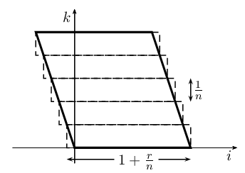
By monotony, this yields

On the other hand, this parallelogram itself covers the rectangles of width , and a similar computation shows that in the limit .

In particular: .

q.e.d. (Theorem encore)

Proving the multidimensional transformation formula for integration by substitution is considerably more difficult than in one dimension, where it basically amounts to reading the chain rule reversedly. Let us state the formula here first:

Theorem (The Transformation Formula, Jacobi): Let be open sets and let be a -diffeomorphism (i.e. exists and both and are -functions). Let be measurable. Then, is measurable and

At the core of the proof is the Theorem on Transformation of Measure that we have proved above. The idea is to approximate by linear mappings, which locally transform the Lebesgue measure underlying the integral and yield the determinant in each point as correction factor. The technical difficulty is to show that this approximation does no harm for the evaluation of the integral.

We will need a lemma first, which carries most of the weight of the proof.

The Preparatory Lemma: Let be open sets and let be a -diffeomorphism. If is a Borel set, then so is , and

Proof: Without loss of generality, we can assume that , and are defined on a compact set . We consider, for instance, the sets

The are open and bounded, is hence compact, and there is a chain for all , with . To each there is, hence, a compact superset on which , and are defined. Now, if we can prove the statement of the Preparatory Lemma on , it will also be true on by the monotone convergence theorem.

As we can consider all relevant functions to be defined on compact sets, and as they are continuous (and even more) by assumption, they are readily found to be uniformly continuous and bounded.

It is obvious that will be a Borel set, as is continuous.

Let us prove that the Preparatory Lemma holds for rectangles with rational endpoints, being contained in .

There is some such that for any , . By continuity, there is a finite constant with

and by uniform continuity, may be chosen small enough such that, for any , even

With this , we may now sub-divide our rectangle into disjoint cubes of side-length such that . In what follows, we shall sometimes need to consider the closure for some of the estimates, but we shall not make the proper distinction for reasons of legibility.

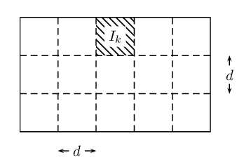
For any given , every other point of may at most have distance in each of its components, which ensures

This, in turn, means, (and has been clear because of the construction of ).

Now, in every of the cubes , we choose the point with

and we define the linear mapping

Remember that for convex sets , differentiable mappings , and points , the mean value theorem shows

Let be a given point in one of the cubes. We apply the mean value theorem to the mapping , which is certainly differentiable, to , and to the convex set :

Note that as , by convexity, and hence the upper estimate of uniform continuity is applicable. Note beyond that, that is the linear mapping and the derivative of a linear mapping is the linear mapping itself.

Now, , as both points are contained in , and hence shows

By continuity (and hence boundedness) of , we also have

which means .

Hence:

Why all this work? We want to bound the measure of the set , and we can get it now: the shift is unimportant by translation invariance. And the set is contained in a cube of side-length . As promised, we have approximated the mapping by a linear mapping on a small set, and the transformed set has become only slightly bigger. By the Theorem on Transformation of Measure, this shows

Summing over all the cubes of which the rectangle was comprised, (remember that is a diffeomorphism and disjoint sets are kept disjoint; besides, has been chosen to be the point in of smallest determinant for )

Taking yields to smaller subdivisions and in the limit to the conclusion. The Preparatory Lemma holds for rectangles.

Now, let be any Borel set, and let . We cover by disjoint (rational) rectangles , such that . Then,

If we let , we see 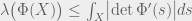$\lambda\bigl(\Phi(X)\bigr)\leq\int_X\bigl|\det\Phi'(s)\bigr|ds$ .

q.e.d. (The Preparatory Lemma)

We didn’t use the full generality that may be possible here: we already focused ourselves on the Borel sets, instead of the larger class of Lebesgue-measurable sets. We shall skip the technical details that are linked to this topic, and switch immediately to the

Proof of Jacobi’s Transformation Formula: We can focus on non-negative functions without loss of generality (take the positive and the negative part separately, if needed). By the Preparatory Lemma, we already have

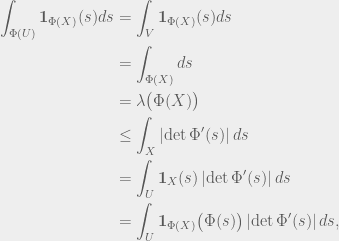
$\displaystyle\begin{aligned} \int_{\Phi(U)}\mathbf{1}_{\Phi(X)}(s)ds &= \int_{V}\mathbf{1}_{\Phi(X)}(s)ds\\ &= \int_{\Phi(X)}ds\\ &= \lambda\bigl(\Phi(X)\bigr)\\ &\leq \int_X\left|\det\Phi'(s)\right|ds\\ &= \int_U\mathbf{1}_X(s)\left|\det\Phi'(s)\right|ds\\ &= \int_U\mathbf{1}_{\Phi(X)}\bigl(\Phi(s)\bigr)\left|\det\Phi'(s)\right|ds, \end{aligned}$

which proves the inequality

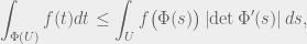
$\displaystyle \int_{\Phi(U)}f(t)dt \leq \int_U f\bigl(\Phi(s)\bigr)\left|\det\Phi'(s)\right|ds,$

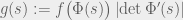
for indicator functions $f = \mathbf{1}_{\Phi(X)}$ . By usual arguments (linearity of the integral, monotone convergence), this also holds for any measurable function . To prove the Transformation Formula completely, we apply this inequality to the transformation and the function $g(s):=f\bigl(\Phi(s)\bigr)\left|\det\Phi'(s)\right|$ :

$\displaystyle \begin{aligned} \int_Uf\bigl(\Phi(s)\bigr)\left|\det\Phi'(s)\right|ds &= \int_{\Phi^{-1}(V)}g(t)dt\\ &\leq \int_Vg\bigl(\Phi^{-1}(t)\bigr)\left|\det(\Phi^{-1})'(t)\right|dt\\ &=\int_{\Phi(U)}f\Bigl(\Phi\bigl(\Phi^{-1}(t)\bigr)\Bigr)\left|\det\Phi'\bigl(\Phi^{-1}(t)\bigr)\right|\left|\det(\Phi^{-1})'(t)\right|dt\\ &=\int_{\Phi(U)}f(t)dt, \end{aligned}$

since the chain rule yields $\Phi'\bigl(\Phi^{-1}\bigr)(\Phi^{-1})' = \bigl(\Phi(\Phi^{-1})\bigr)' = \mathrm{id}$ . This means that the reverse inequality also holds. The Theorem is proved.

q.e.d. (Theorem)

There may be other, yet more intricate proofs of this Theorem. We shall not give any other of them here, but the rather mysterious looking way in which the determinant pops up in the transformation formula is not the only way to look at it. There is a proof by induction, given in Heuser’s book, where the determinant just appears from the inductive step. However, there is little geometric intuition in this proof, and it is by no means easier than what we did above (as it make heavy use of the theorem on implicit functions). Similar things may be said about the rather functional analytic proof in Königsberger’s book (who concludes the transformation formula by step functions converging in the $L^1$ -norm, he found the determinant pretty much in the same way that we did).

Let us harvest a little of the hard work we did on the Transformation Formula. The most common example is the integral of the standard normal distribution, which amounts to the evaluation of

$\displaystyle \int_{-\infty}^\infty e^{-\frac12x^2}dx.$

This can happen via the transformation to polar coordinates:

$\Phi:(0,\infty)\times(0,2\pi)\to\mathbb{R}^2,\qquad (r,\varphi)\mapsto (r\cos \varphi, r\sin\varphi).$

For this transformation, which is surjective on all of $\mathbb{R}^2$ except for a set of measure $0$ , we find

$\Phi'(r,\varphi) = \begin{pmatrix}\cos\varphi&-r\sin\varphi\\\sin\varphi&\hphantom{-}r\cos\varphi\end{pmatrix},\qquad \det\Phi'(r,\varphi) = r.$

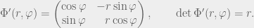
From the Transformation Formula we now get

$\displaystyle \begin{aligned} \left(\int_{-\infty}^\infty e^{-\frac12x^2}dx\right)^2 &= \int_{\mathbb{R}^2}\exp\left(-\frac12x^2-\frac12y^2\right)dxdy\\ &= \int_{\Phi\left((0,\infty)\times(0,2\pi)\right)}\exp\left(-\frac12x^2-\frac12y^2\right)dxdy\\ &= \int_{(0,\infty)\times(0,2\pi)}\exp\left(-\frac12r^2\cos^2(\varphi)-\frac12r^2\sin^2(\varphi)\right)\left|\det\Phi'(r,\varphi)\right|drd\varphi\\ &= \int_{(0,\infty)\times(0,2\pi)}\exp\left(-\frac12r^2\right)rdrd\varphi\\ &= \int_0^\infty\exp\left(-\frac12r^2\right)rdr\int_0^{2\pi}d\varphi \\ &= 2\pi \left[-\exp\left(-\frac12r^2\right)\right]_0^\infty\\ &= 2\pi \left(1-0\right)\\ &= 2\pi. \end{aligned}$

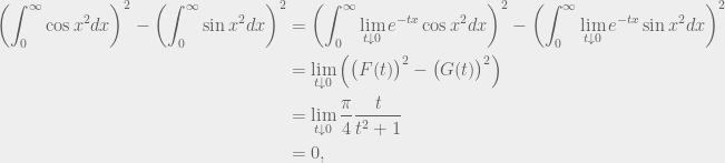
In particular, $\int_{-\infty}^\infty e^{-\frac12x^2}dx=\sqrt{2\pi}$ . One of the very basic results in probability theory.

Another little gem that follows from the Transformation Formula are the Fresnel integrals

$\displaystyle \int_{0}^\infty \cos(x^2)dx = \int_{0}^\infty\sin(x^2)dx = \sqrt{\frac{\pi}{8}}.$

They follow from the same basic trick given above for the standard normal density, but as other methods for deriving this result involve even trickier uses of similarly hard techniques (the Residue Theorem, for instance, as given in Remmert’s book), we shall give the proof of this here:

Consider

$\displaystyle F(t)=\int_{0}^\infty e^{-tx^2}\cos(x^2)dx\qquad\text{and}\qquad\int_{0}^\infty e^{-tx^2}\sin(x^2)dx.$

Then, the trigonometric identity $\cos a+b = \cos a \cos b - \sin a\sin b$ tells us

$\displaystyle \begin{aligned} \bigl(F(t)\bigr)^2 - \big(G(t)\bigr)^2 &= \int_0^\infty\int_0^\infty e^{-t(x^2+y^2)}\cos(x^2)\cos(y^2)dxdy - \int_0^\infty\int_0^\infty e^{-t(x^2+y^2)}\sin(x^2)\sin(y^2)dxdy\\ &= \int_0^\infty\int_0^\infty e^{-t(x^2+y^2)}\bigl(\cos(x^2+y^2)+\sin(x^2)\sin(y^2) - \sin(x^2)\sin(y^2)\bigr)dxdy\\ &= \int_0^\infty\int_0^{\frac\pi2}e^{-tr^2}\cos(r^2)rd\varphi dr\\ &= \frac\pi2 \int_0^\infty e^{-tu}\cos u\frac12du. \end{aligned}$

This integral can be evaluated by parts to show

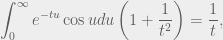
$\displaystyle \int_0^\infty e^{-tu}\cos udu\left(1+\frac1{t^2}\right) = \frac1t,$

which means

$\displaystyle \bigl(F(t)\bigr)^2 - \bigl(G(t)\bigr)^2 = \frac\pi4\int_0^\infty\int_0^\infty e^{-tu}\cos udu = \frac\pi4\frac t{t^2+1}.$

Then we consider the product $F(t)G(t)$ and use the identity $\sin(a+b) = \cos a\sin b + \cos b\sin a$ , as well as the symmetry of the integrand and integration by parts, to get

$\displaystyle \begin{aligned} F(t)G(t) &= \int_0^\infty\int_0^\infty e^{-t(x^2+y^2)}\bigl(\cos(x^2)\sin(y^2)\bigr)dxdy\\ &=2\int_0^\infty\int_0^ye^{-t(x^2+y^2)}\sin(x^2+y^2)dxdy\\ &=2\int_0^\infty\int_0^{\frac\pi8}e^{-tr^2}\sin(r^2)rd\varphi dr\\ &=\frac\pi4\int_0^\infty e^{-tr^2}\sin(r^2)r dr\\ &=\frac\pi4\int_0^\infty e^{-tu}\sin u\frac12du\\ &=\frac\pi8\frac1{1+t^2}. \end{aligned}$

We thus find by the dominated convergence theorem

$\displaystyle \begin{aligned} \left(\int_0^\infty\cos x^2dx\right)^2-\left(\int_0^\infty\sin x^2dx\right)^2 &= \left(\int_0^\infty\lim_{t\downarrow0}e^{-tx}\cos x^2dx\right)^2-\left(\int_0^\infty\lim_{t\downarrow0}e^{-tx}\sin x^2dx\right)^2 \\ &=\lim_{t\downarrow0}\left(\bigl(F(t)\bigr)^2-\bigl(G(t)\bigr)^2\right)\\ &=\lim_{t\downarrow0}\frac\pi4\frac{t}{t^2+1}\\ &=0, \end{aligned}$

and

$\displaystyle \begin{aligned} \left(\int_0^\infty\cos x^2dx\right)^2 &= \left(\int_0^\infty\cos x^2dx\right)\left(\int_0^\infty\sin x^2dx\right)\\ &=\left(\int_0^\infty\lim_{t\downarrow0}e^{-tx}\cos x^2dx\right)\left(\int_0^\infty\lim_{t\downarrow0}e^{-tx}\sin x^2dx\right)\\ &=\lim_{t\downarrow0}F(t)G(t)\\ &=\lim_{t\downarrow0}\frac\pi8\frac1{1+t^2}\\ &=\frac\pi8. \end{aligned}$

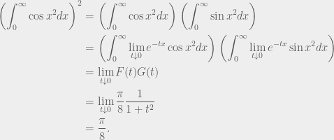
One can easily find the bound that both integrals must be positive and from the first computation, we get

$\int_0^\infty\cos x^2dx = \int_0^\infty\sin x^2dx,$

from the second computation follows that the integrals have value $\sqrt{\frac\pi8}$ .

q.e.d. (Fresnel integrals)

Even Brouwer’s Fixed Point Theorem may be concluded from the Transformation Formula (amongst a bunch of other theorems, none of which is actually as deep as this one though). This is worthy of a seperate text, mind you.

Advertisements Share this:

Twitter
Facebook
Google

Like this:Like Loading...