One of the most important things to do when working with a lot of data is to reduce the dimensionality of that data as far as possible. When the data you are working with is text, this is done by reducing the number of words used in the corpus without compromising the meaning of the text.
One of the most fascinating things about language was discovered by G K Zipf in 1935¹: that the most frequently used words in (the English) language are actually few in number, and obey a ‘power law’. The most frequently used word occurs twice as often as the next most frequently word, three times as often as the third, and so on. Zipf’s law forms a curve like this:
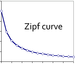 The distribution seems to apply to languages other than English, and it’s been tested many times, including using the text of, for example, novels. It seems we humans are very happy to come up with a rich and varied lexography, but then rely on just a few to communicate with each other. This makes perfect sense as far as I can see: I say I live on a boat, gets the essentials across (a thing that floats, a bit of an alternative lifestyle, how cool am I? etc.) because were I to say I live on a lifeboat, I then have to explain that it’s like one of the fully-enclosed ones you see hanging from the side of cruise ships, not the open Titanic-style ones most people would imagine.
“For language in particular, any such account of the Zipf’s law provides a psychological theory about what must be occurring in the minds of language users. Is there a multiplicative stochastic process at play? Communicative optimization? Preferential reuse of certain forms?” (Piantadosi, 2014)
A recent paper by Piantadosi² reviewed some of the research on word frequency distributions, and concluded that, although Zipf’s law holds broadly true, there are other models that provide a more reliable picture of word frequency which depend on the corpus selected. Referring to a paper by another researcher, he writes “Baayen finds, with a quantitative model comparison, that which model is best depends on which corpus is examined. For instance, the log-normal model is best for the text The Hound of the Baskervilles, but the Yule–Simon model is best for Alice in Wonderland.”
I’m not a mathematician, but that broadly translates as ‘there are different ways of calculating word frequency, you pays your money you takes your choice”. Piantadosi then goes on to explain the problem with Zipf’s law: it doesn’t take account of the fact that some words may occur more frequently that others purely by chance, giving the illusion of an underlying structure where none may exist. He then goes on to suggests a way to overcome this problem, which is to use two independent corpora, or split a corpora in half and then test word frequency distribution in each. He then tests a range of models, and concludes that the “…distribution in language is only near-Zipfian.” and concludes “Therefore, comparisons between simple models will inevitably be between alternatives that are both “wrong.” “.
Semantics also has a strong influence on word frequency. Piantadosi cites a study³ that compared 17 languages across six language families and concluded that simple words are used with greater frequency in all of them, and result in a near-Zipfian model. More importantly for my project, he notes that other studies indicate that word frequencies are domain-dependent. Piantadosi’s paper is long and presents a very thorough review of research relating to Zipf’s law, but the main point is that it does exist, even though why it should be so is still unclear. The next question is should the most frequently used words from a particular domain also be removed?
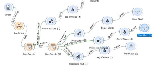
As I mentioned before, research has already established that it’s worth removing (at least as far as English is concerned) a selection of words. Once that’s done, which are the most frequently used words in my data? I used Orange is to split my data in half and generate three word clouds based on the same parameters, and observe the result. Of course I’m not measuring the distribution of words, I’m just doing a basic word count and then displaying the results, but it’s a start. First, here’s my workflow:
I’ve shuffled (randomised) my corpus, taken a training sample of 25%, and then split this again into two equal samples. Each of these has been pre-processed using the following parameters:
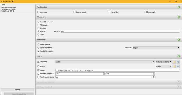
Pre-processing parameters. I used the lemmatiser this time.
The stop word set is the extended set of ‘standard’ stop words used by Scikit that I referred to in my previous post, plus a few extra things to try and get rid of some of the rubbish that appears.
The word clouds for the full set, and each separate sample, look like this:

Complete data set (25% sample, 2316 rows)

50% of sample (1188 rows)

Remaining 50% of sample
The graph below plots the frequency with which the top 500 words occur.

So, I can conclude that based on word counts, each of my samples is similar to each other, and to the total (sampled) corpus. This is good.
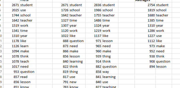
So, should I remove the most frequently used words, and if so, how many? Taking the most frequently used words across each set, and calculating the average for each word, gives me a list as follows:
And if I take them out, the word cloud (based on the entire 25% set) looks like this:

Which leads me to think I should take ‘learning’ and ‘teaching’ out as well. It’s also interesting that the word ‘pupil’ has cropped up here – I wonder how many teachers still talk about pupils rather than students? Of course, this data set contains blogs that may be a few years old, and/or be written by bloggers who prefer the term. Who knows? In fact, Orange can tell me. The ‘concordance’ widget, when connected to the bag of words, tells me that ‘pupil’ is used in 64 rows (blogs) and will show me a snippet of the sentence.

It’s actually used a total of 121 times, and looking at the context I’m not convinced it adds value in terms of helping me with my ultimate goal, which is clustering blog posts by topic, so it’s probably worth mentioning here that the words used the least often are going to be the most numerically relevant when it comes to grouping blogs by topic.

Could I take out some more? This is a big question. I don’t want to remove so many words that the data becomes difficult to cluster. Think of this as searching the blog posts using key words, much as you would when you search Google. Where, as a teacher, you might want to search ‘curriculum’, you might be more interesting in results that discuss ‘teaching (the) curriculum’ rather than those that cover ‘designing (the) curriculum’. If ‘teaching’ has already been removed, how will you find what you’re looking for? Alternatively, does it matter so long as search returns everything that contains the word ‘curriculum’? You may be more interested in searching for ‘curriculum’ differentiating by key stage. For my purposes, I think I’d be happy with a cluster labelled ‘curriculum’ that covered all aspects of the topic. I’ll be able to judge when I see some actual clusters emerge, and have the chance to examine them more closely. Which, incidentally, the concordance widget tells me is used in 93 blogs, and appears 147 times. That’s more than ‘pupil’, but because of my specialised domain knowledge I judge to be more important to the corpus.
Which is also a good example of researcher bias.